
Table of Contents
2 May 2020
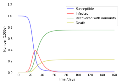
Modified SIR Model (SIRD model)
When I was going through the traditional SIR your model I had a few observations
- they have only consider the Recovery Rate only and not Death Rate
- the current model does not mimic the current situation
As for any epidemic it is a very common thing that there will be some Infected people who will be recovered and some people will be deceased. So the traditional model tackles an optimal situation where all infected will be recovered at the end of the time. So I have modified the current mathematical model to incorporate the death rate in terms of infected people.
This has two main advantages the first one being the modified model is extremely close to a real life situation where a normal people is susceptible for a disease then he/she gets infected then either he/she recovers or dies from the . Keeping this situation in mind I have added death component over time t.
This this epidemic model handles a real life situation. When we plug in the Infection rate, death rate, recover rate we can find out how the trend of this epidemic will look like for a particular Territory or a state or a country.
Mathematical Background
Let N be the size of the total population.
Then,
$\displaystyle S(t) + I(t) + R(t) + D(t) = N$
The Modified SIR system be expressed by the following set of ordinary differential equations:
$\displaystyle \frac{dS}{dt} =-\beta SI$
$\displaystyle \frac{dI}{dt} =\beta SI - \gamma I - \alpha I$
$\displaystyle \frac{dR}{dt} =\gamma I$
$\displaystyle \frac{dD}{dt} =\alpha I$
Python Code to Implement Modified SIR Model
from scipy.integrate import odeint
import matplotlib.pyplot as plt

# Total population, N.
N = 10000
# Initial number of infected and recovered individuals, I0 and R0.
I0, R0, D0 = 1, 0, 0
# Everyone else, S0, is susceptible to infection initially.
S0 = N - I0 - R0 - D0
# Contact rate, beta, and mean recovery rate, gamma, (in 1/days).
alpha, beta, gamma = 0.03, 0.5, 1./10
# A grid of time points (in days)
t = np.linspace(0, 160, 160)

# The SIR model differential equations.
def deriv(y, t, N, beta, gamma, alpha):
    S, I, R, D = y
    dSdt = -beta * S * I / N
    dIdt = beta * S * I / N - gamma * I - alpha * I
    dRdt = gamma * I
    dDdt = alpha * I
    return dSdt, dIdt, dRdt, dDdt

# Initial conditions vector
y0 = S0, I0, R0, D0
# Integrate the SIR equations over the time grid, t.
ret = odeint(deriv, y0, t, args=(N, beta, gamma, alpha))
S, I, R, D = ret.T

# Plot the data on three separate curves for S(t), I(t) and R(t)
fig = plt.figure(facecolor='w')
ax = fig.add_subplot(111, axisbelow=True)
ax.plot(t, S/N, 'b', alpha=0.5, lw=2, label='Susceptible')
ax.plot(t, I/N, 'r', alpha=0.5, lw=2, label='Infected')
ax.plot(t, R/N, 'g', alpha=0.5, lw=2, label='Recovered with immunity')
ax.plot(t, D/N, 'y', alpha=0.5, lw=2, label='Death')

ax.set_xlabel('Time /days')
ax.set_ylabel('Number (1000s)')
ax.set_ylim(0,1.2)
ax.yaxis.set_tick_params(length=0)
ax.xaxis.set_tick_params(length=0)
ax.grid(b=True, which='major', c='w', lw=2, ls='-')
legend = ax.legend()
legend.get_frame().set_alpha(0.5)
for spine in ('top', 'right', 'bottom', 'left'):
    ax.spines[spine].set_visible(False)
plt.show()
Output:
15 April 2020
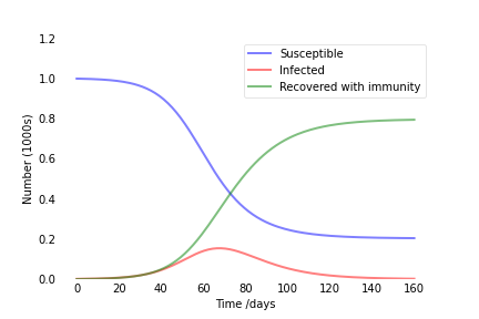
The SIR Model
The SIR model is one of the simplest compartmental models, and many models are derivatives of this basic form.
The model consists of three compartments:
- S for the number of susceptible,
- I for the number of infectious, and
- R for the number of recovered or deceased (or immune) individuals.
This model is reasonably predictive for infectious diseases which are transmitted from human to human, and where recovery confers lasting resistance, such as measles, mumps and rubella.
These variables ( S , I, and R) represent the number of people in each compartment at a particular time. To represent that the number of susceptible, infected and recovered individuals may vary over time (even if the total population size remains constant), we make the precise numbers a function of t(time): S(t), I(t) and R(t). For a specific disease in a specific population, these functions may be worked out in order to predict possible outbreaks and bring them under control.
(Source: Wikipedia)
Mathematical Background
Let N be the size of the total population.
Then,
$\displaystyle S(t) + I(t) + R(t) = N$
The SIR system be expressed by the following set of ordinary differential equations:
$\displaystyle \frac{dS}{dt} =-\beta SI$
$\displaystyle \frac{dI}{dt} =\beta SI - \gamma I$
$\displaystyle \frac{dR}{dt} =\gamma I$
Python Code to Implement Traditional SIR Model
from scipy.integrate import odeint
import matplotlib.pyplot as plt
import numpy as np


# Total population, N.
N = 1000
# Initial number of infected and recovered individuals, I0 and R0.
I0, R0 = 1, 0
# Everyone else, S0, is susceptible to infection initially.
S0 = N - I0 - R0
# Contact rate, beta, and mean recovery rate, gamma, (in 1/days).
beta, gamma = 0.2, 1./10
# A grid of time points (in days)
t = np.linspace(0, 160, 160)

# The SIR model differential equations.
def deriv(y, t, N, beta, gamma):
    S, I, R = y
    dSdt = -beta * S * I / N
    dIdt = beta * S * I / N - gamma * I
    dRdt = gamma * I
    return dSdt, dIdt, dRdt

# Initial conditions vector
y0 = S0, I0, R0
# Integrate the SIR equations over the time grid, t.
ret = odeint(deriv, y0, t, args=(N, beta, gamma))
S, I, R = ret.T

# Plot the data on three separate curves for S(t), I(t) and R(t)
fig = plt.figure(facecolor='w')
ax = fig.add_subplot(111, axisbelow=True)
ax.plot(t, S/1000, 'b', alpha=0.5, lw=2, label='Susceptible')
ax.plot(t, I/1000, 'r', alpha=0.5, lw=2, label='Infected')
ax.plot(t, R/1000, 'g', alpha=0.5, lw=2, label='Recovered with immunity')
ax.set_xlabel('Time /days')
ax.set_ylabel('Number (1000s)')
ax.set_ylim(0,1.2)
ax.yaxis.set_tick_params(length=0)
ax.xaxis.set_tick_params(length=0)
ax.grid(b=True, which='major', c='w', lw=2, ls='-')
legend = ax.legend()
legend.get_frame().set_alpha(0.5)
for spine in ('top', 'right', 'bottom', 'left'):
    ax.spines[spine].set_visible(False)
plt.show()
Output:
30 March 2020
COVID-19 Website
I have built this website to see the trend for all types of cases over time.
References
- https://scipython.com/book/chapter-8-scipy/additional-examples/the-sir-epidemic-model/
- https://web.stanford.edu/~chadj/sird-paper.pdf