These concepts form the foundation for causal inference, enabling applications across science, economics, and machine learning. Let me know if you’d like further clarification or examples!
- Structural Causal Models (SCMs)
- Do-Calculus
- Advanced Topics in SCMs and Do-Calculus
- References
Structural Causal Models (SCMs)
SCMs are mathematical models used to describe and reason about causal systems. An SCM consists of variables, their causal relationships, and equations describing those relationships.
Components of an SCM
An SCM \(M\) is defined as:
- Endogenous variables (\(X, Y, Z, ...\)): Variables determined within the system.
- Exogenous variables (\(U\)): Variables external to the system that influence endogenous variables.
-
Structural equations: Deterministic or stochastic functions mapping the relationship between variables.
$ X = f_X(U_X, \text{Parents}(X)) $
- Causal graph (DAG): A directed acyclic graph representing causal relationships.
Example of an SCM
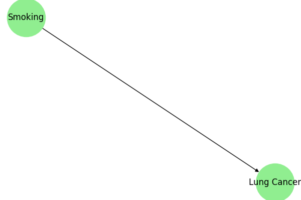
Let’s model the effect of smoking (\(S\)) on lung cancer (\(C\)):
- Exogenous variables: Genetic predisposition (\(U\)).
-
Structural equations:
$ S = f_S(U_S), \quad C = f_C(S, U_C) $
-
Graph:
$ S \rightarrow C $
Python Example: Visualizing an SCM
import networkx as nx
import matplotlib.pyplot as plt

# Define SCM graph
scm = nx.DiGraph()
scm.add_edges_from([("Smoking", "Lung Cancer")])

# Visualize
plt.figure(figsize=(6, 4))
nx.draw(scm, with_labels=True, node_color='lightgreen', node_size=3000, font_size=12)
plt.title("Simple SCM for Smoking and Lung Cancer")
plt.show()

Assumptions in SCMs
- Causal Markov Assumption: Each variable is independent of its non-effects given its direct causes.
- Faithfulness: Observed independencies reflect true causal structure.
SCMs and Causal Queries
- Prediction: What happens to \(Y\) if \(X\) changes naturally?
- Intervention: What happens to \(Y\) if \(X\) is forcibly set to a specific value (\(do(X = x)\))?
- Counterfactuals: What would \(Y\) have been if \(X\) had taken a different value?
Do-Calculus
Do-Calculus is a formal framework introduced by Judea Pearl to manipulate and evaluate interventions in causal systems. It allows us to answer causal questions by reasoning about the effects of interventions using observational data.
The Do-Operator
The \(do(X = x)\) operator represents an intervention that forces \(X\) to take the value \(x\), disconnecting \(X\) from its natural causes.
-
Observational probability:
$ P(Y|X) $ Represents the distribution of \(Y\) given \(X\) in a natural setting.
-
Interventional probability:
$ P(Y|do(X = x)) $ Represents the distribution of \(Y\) when \(X\) is externally set to \(x\), irrespective of \(X\)’s natural causes.
Rules of Do-Calculus
Do-Calculus consists of three rules for transforming probabilities with interventions:
Rule 1: Ignoring Observations
If \(X\) is independent of \(Y\) given \(Z\) in the causal graph after removing incoming edges to \(X\), then:
$ P(Y|do(X), Z) = P(Y|Z) $
Rule 2: Action/Observation Exchange
If \(Y\) is independent of \(X\) given \(Z\) in the modified causal graph where incoming edges to \(X\) are removed, then:
$ P(Y|do(X), Z) = P(Y|X, Z) $
Rule 3: Removing Actions
If \(X\) is independent of \(Y\) in the modified graph obtained by removing outgoing edges from \(X\), then:
$ P(Y|do(X)) = P(Y) $
Applications of Do-Calculus
Application 1: Identifying Causal Effects
Do-Calculus helps compute:
$ P(Y|do(X = x)) $ Even when direct experimentation is not possible.
Application 2: Mediation Analysis
It quantifies how much of the effect of \(X\) on \(Y\) is mediated through an intermediate variable \(M\).
Example: Smoking and Lung Cancer
-
Observational probability:
$ P(C | S) $ This includes confounding due to genetic predisposition.
-
Interventional probability:
$ P(C | do(S = 1)) $ This isolates the causal effect of smoking.
Python Example: Estimating \(do(X)\)
from dowhy import CausalModel
import pandas as pd

# Sample data
data = pd.DataFrame({
    'Smoking': [0, 1, 1, 0, 1],
    'Lung Cancer': [0, 1, 1, 0, 1],
    'Genetics': [1, 0, 1, 0, 1]
})

# Define causal model
model = CausalModel(
    data=data,
    treatment='Smoking',
    outcome='Lung Cancer',
    common_causes=['Genetics']
)

# Identify causal effect
identified_estimand = model.identify_effect()
print(identified_estimand)
Output:
### Estimand : 1
Estimand name: backdoor
Estimand expression:
    d
──────────(E[Lung Cancer|Genetics])
d[Smoking]
Estimand assumption 1, Unconfoundedness: If U→{Smoking} and U→Lung Cancer then P(Lung Cancer|Smoking,Genetics,U) = P(Lung Cancer|Smoking,Genetics)

### Estimand : 2
Estimand name: iv
No such variable(s) found!

### Estimand : 3
Estimand name: frontdoor
No such variable(s) found!
Advanced Topics in SCMs and Do-Calculus
Counterfactual Reasoning in SCMs
Counterfactuals evaluate what could have happened under alternative scenarios. SCMs enable counterfactual queries by:
- Fixing exogenous variables.
- Modifying structural equations.
Example: If a patient had taken the drug, what would their outcome have been?
Transportability
Transportability uses Do-Calculus to generalize causal knowledge from one population to another with different causal structures.
Combining SCMs with Machine Learning
Modern research integrates SCMs with machine learning to:
- Learn causal structures from data.
- Predict causal effects using observational data.
Python Example: Learning Causal Graphs with CausalNex
from causalnex.structure import StructureModel

# Create structure model
sm = StructureModel()
sm.add_edges_from([
    ('Smoking', 'Lung Cancer'),
    ('Genetics', 'Lung Cancer')
])

# Visualize
from causalnex.plots import plot_structure
plot_structure(sm, graph_attributes={"scale": "2"})
References
- Judea Pearl (2000). Causality: Models, Reasoning, and Inference.
- Morgan and Winship (2015). Counterfactuals and Causal Inference.
- Spirtes, Glymour, and Scheines (2001). Causation, Prediction, and Search.
- DoWhy Documentation: https://microsoft.github.io/dowhy/
- CausalNex Documentation: https://causalnex.readthedocs.io/
